By: Arthur Calvi (Intern at Kayrros, supervised by Aurélien De Truchis, 2022)
Introduction & Inspiration
In 2022, I joined Kayrros as an intern under the supervision of Aurélien De Truchis with a mission: adapt and enhance the Google Dynamic World approach for robust, high-resolution land use and land cover classification.
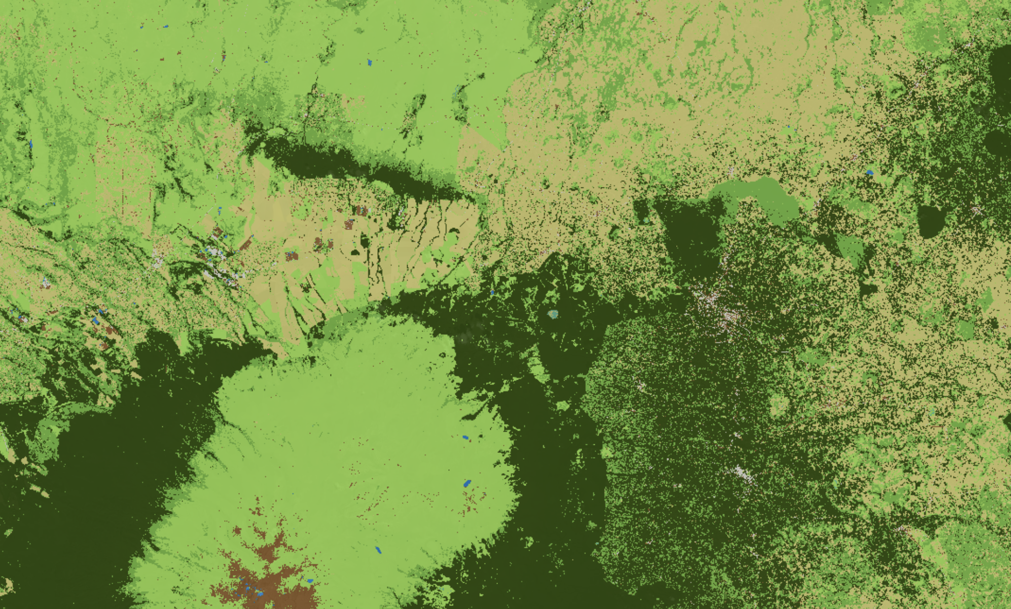
Google Dynamic World is an AI-driven, 10 m resolution, near real-time land cover dataset that categorizes Earth into nine classes: Water, Trees, Grass, Crops, Shrub & Scrub, Flooded Vegetation, Built-Up Area, Bare Ground, and Snow & Ice. While Dynamic World is already remarkable, it sometimes struggles with temporal consistency and certain niche environments. My work at Kayrros aimed at making a lightweight yet robust deep learning pipeline that can handle multiple satellite data sources across biomes and seasons.
Method Overview
My project drew from the U-Net family of CNN architectures, famous for its success in medical imaging and remote sensing. However, I employed specific modifications to meet production constraints and further improve consistency over time:
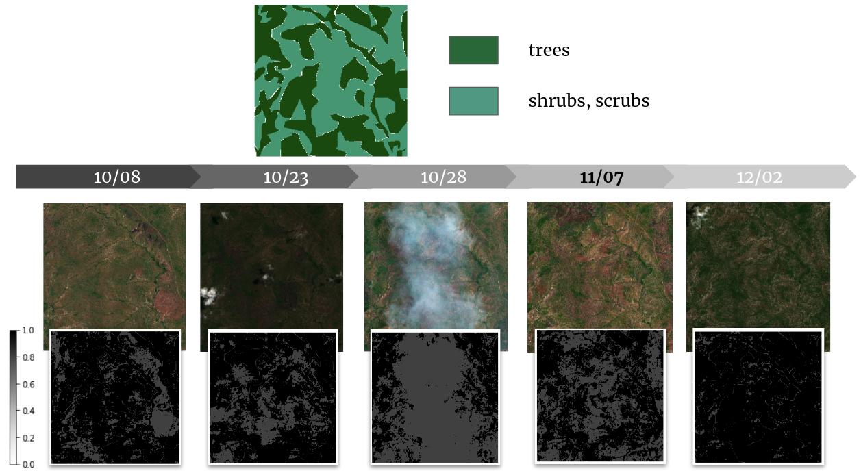
- Data Preparation & Augmentation: I used a "temporal augmentation" trick, ensuring multiple satellite images captured at different dates fed the same label (with refined confidence). This step helped train the model to remain robust against changing vegetation cycles and atmospheric effects.
- Specialized Inputs: Beyond the standard RGB and near-infrared bands, I included derived indices (like NDVI, NDMI) and SRTM30-based elevation data to add extra context. This proved helpful for challenging distinctions such as Crops vs. Grass, or Trees vs. Shrubs.
- Lightweight Architecture: I built a minimal U-Net variant with only three downsampling levels, plus carefully chosen enhancements like attention gates or atrous spatial pyramid pooling. This balanced inference speed (for large-scale production) and accuracy.
- Global Reach & Satellite Agnosticism: By systematically normalizing data from Sentinel-2, Landsat-8, and older Landsat missions, the model remains flexible enough to be used for historical analyses and near real-time applications.
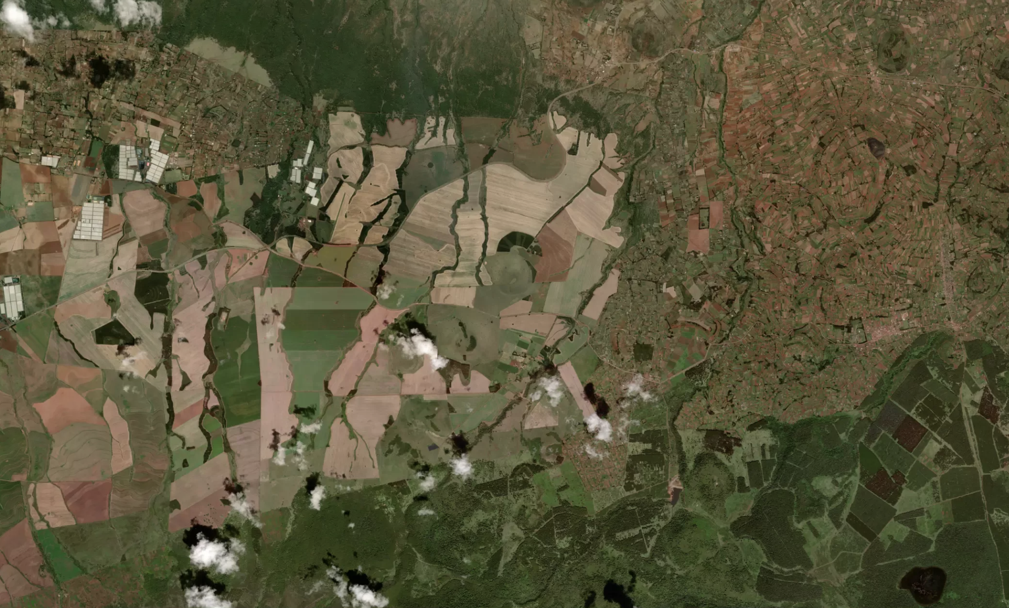
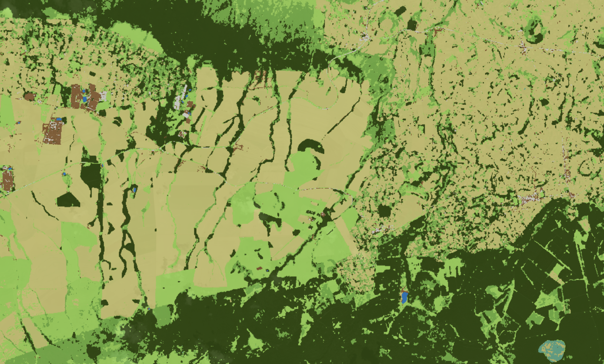
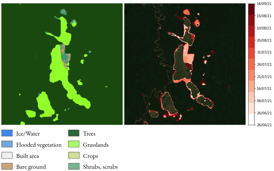
Interactive Slider Explanation
Below, you can see how the model transforms a raw Sentinel-2 input (left side) into a land cover classification (right side). Drag the slider to compare the images.
Results & Benchmarks
My approach was tested across multiple biomes—from temperate forests to tropical regions—totaling 14 major ecoregions. Our final model achieved strong performance metrics with 46.9% accuracy, 31.8% IoU (Intersection over Union), and 75.1% MCC (Matthews Correlation Coefficient). Most importantly, these results remained consistent across different biomes—a crucial feature for Kayrros, whose assets span diverse geographical regions worldwide. While our metrics remained slightly below Google Dynamic World's performance, we successfully built a lightweight and temporally consistent alternative.
Impact & Conclusion
This internship project at Kayrros resulted in a production-ready deep learning pipeline for reliable land cover mapping. By leveraging smart data augmentation, additional satellite indices, and a lightweight architecture, the solution demonstrated strong temporal consistency across diverse geographies.
The model proved particularly effective for deriving dynamic indicators such as deforestation alerts, agricultural expansion, and other environmental monitoring applications. While not quite matching Dynamic World's accuracy, our approach offered improved temporal consistency and multi-satellite compatibility.
Acknowledgement: This project was conducted as part of my 2022 internship at Kayrros, under the supervision of Aurélien De Truchis.