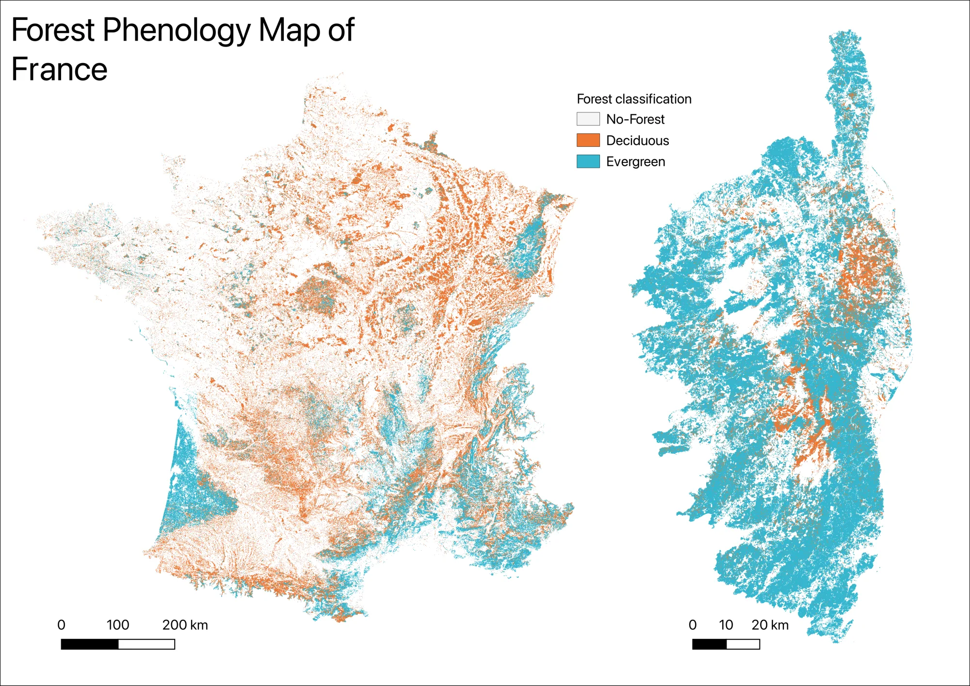
The full method and results are available in the working manuscript (PDF).
Podcast version of this article (NotebookLM)
Deciduous and evergreen forests do not reflect light in the same way through the year. During my PhD, I used that seasonal signal to build a compact representation of irregular Sentinel-2 time series. The representation was interpretable and cheap to train on, but it depended on features designed by hand.
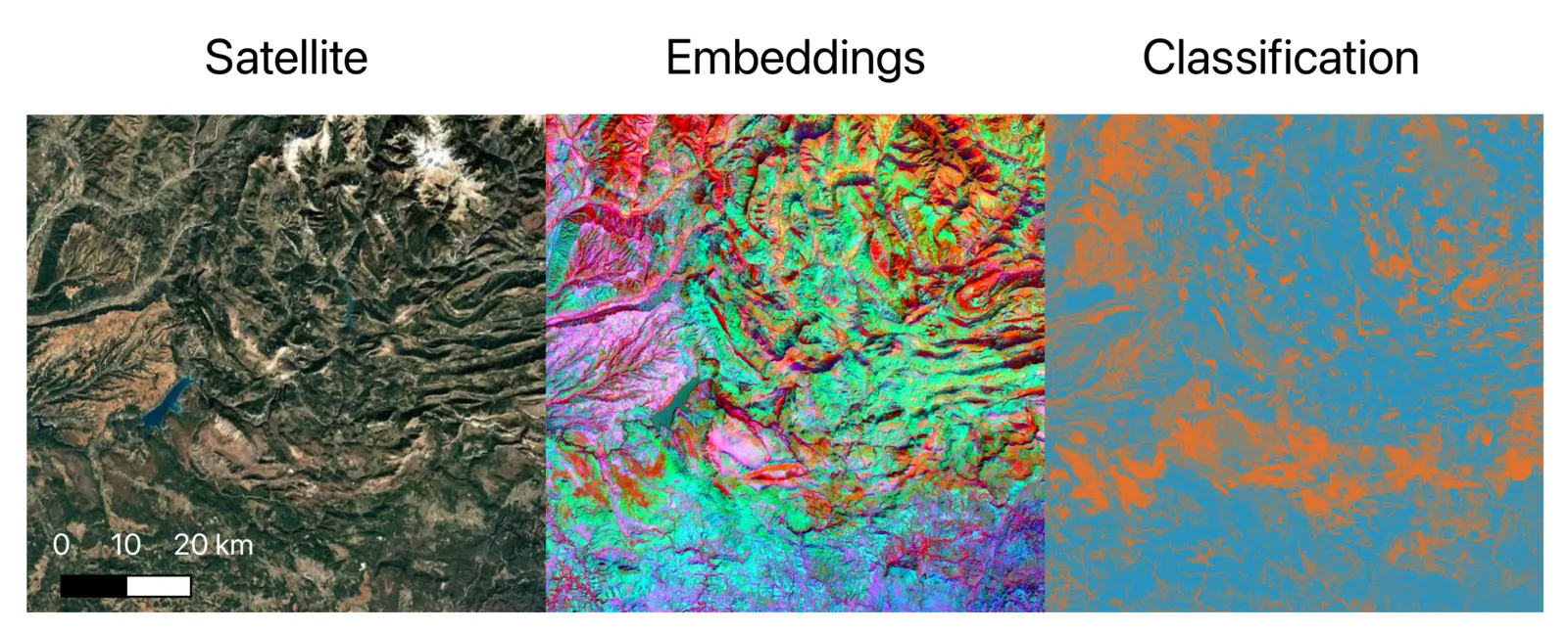
When Google and Google DeepMind released AlphaEarth Foundations and its annual Satellite Embedding dataset, I revisited the same task. I kept the labels, spatial folds, feature budget, and lightweight classifiers fixed. Only the representation changed. Because the embeddings were precomputed, the downstream experiment required no local GPU training.
This is an unpublished working manuscript, not a peer-reviewed paper. I am its sole author. Alexandre d’Aspremont, Sarah Brood, and Philippe Ciais reviewed drafts and helped me refine the methodology.
Browse the research code and experiment material.
Across three classifiers, mean macro-F1 increased from 0.860 to 0.897. The embedding maps were also better calibrated and much less fragmented, without spatial smoothing after classification.
This study was one part of a broader PhD on detecting, segmenting, and classifying forest disturbances from satellite imagery. Phenology mattered because normal seasonal variation can otherwise be confused with abnormal change in satellite time series. The companion article, Joining forest disturbance records with graph theory, describes how I combined incomplete event records before attempting to build that disturbance dataset.
One task, two representations
Sentinel-2 observes the same place every few days. After cloud masking, those observations form a seasonal curve: deciduous canopies green up in spring and lose their leaves in autumn, while evergreen canopies tend to vary less.
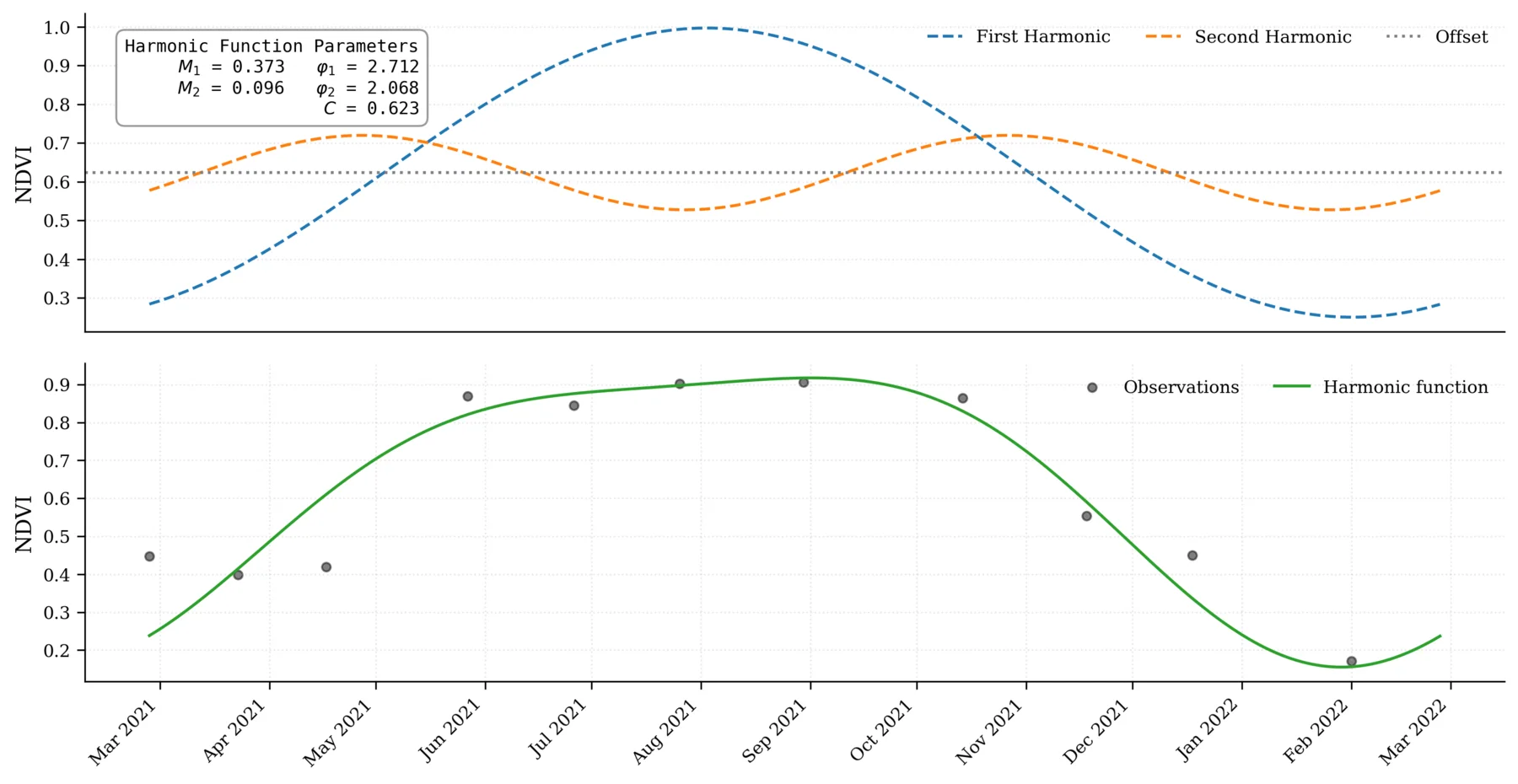
For the handcrafted baseline, I computed four vegetation indices: NDVI, EVI, NBR, and CRSWIR. I then fitted a two-harmonic model over one annual cycle of each index, using 12- and 6-month components:
\[z(t) = c + \sum_{k=1}^{2}\left[a_k \cos\left(\frac{2\pi kt}{T}\right) + b_k \sin\left(\frac{2\pi kt}{T}\right)\right] + \varepsilon(t)\]This turns a noisy year of observations into a compact description: average greenness, the strength and timing of seasonal variation, and the error left unexplained. Starting from 32 candidates, recursive feature elimination inside the training tiles of each fold retained 14. I call this representation HARM-14.
The alternative started from AlphaEarth’s 64-dimensional annual embeddings at 10 m resolution. These embeddings summarize spectral, temporal, and local spatial information learned upstream from a much larger satellite archive. The same selection procedure retained 14 dimensions, producing EMB-14. Matching the feature count kept the main benchmark deliberately conservative; higher-dimensional embedding variants were examined separately in the manuscript.
A controlled benchmark
The reference data contained 14.1 million labelled forest pixels across metropolitan France. About 88.6% came from photo-interpreted polygons in IGN’s BD Forêt, and 11.4% came from field or expert sources. I applied a 100 m inward buffer to the BD Forêt polygons before sampling, reducing mixed pixels near their boundaries.
The pixels were grouped into 639 non-overlapping tiles, each 2.5 km wide, distributed across 11 ecological regions. Five-fold cross-validation was stratified by ecological region. No tile contributed pixels to both training and validation in the same fold, reducing leakage from local spatial autocorrelation.
I trained logistic regression, a linear SVM, and a random forest. The folds, class weights, and training samples were the same for both representations. Hyperparameters were selected on the harmonic baseline and transferred unchanged to the embeddings. This was not a larger model competing with a smaller one; only the model’s view of the satellite data changed.
Across the three classifiers, macro-F1 increased from 0.860 with harmonics to 0.897 with embeddings, a gain of 3.7 percentage points. With the random forest, it rose from 0.874 to 0.905. In a separate 28-feature fusion diagnostic on the intersection of valid pixels, adding the harmonic features moved random-forest macro-F1 from 0.905 to 0.908. That small gain suggests limited complementarity, but it is not the same fixed-complexity comparison as HARM-14 versus EMB-14.
The map changed more than the score
The numerical gain was useful, but the maps were more revealing. Raw embedding predictions produced larger contiguous regions and fewer isolated class changes. Compared with the harmonic model, edge density fell by 55% and patch density by 65%, without morphological smoothing.
The probabilities were also better calibrated. Expected calibration error fell from 0.059 to 0.033. In practice, the confidence attached to a prediction was closer to its observed reliability, which matters when a map will later be reviewed, thresholded, or combined with other evidence.
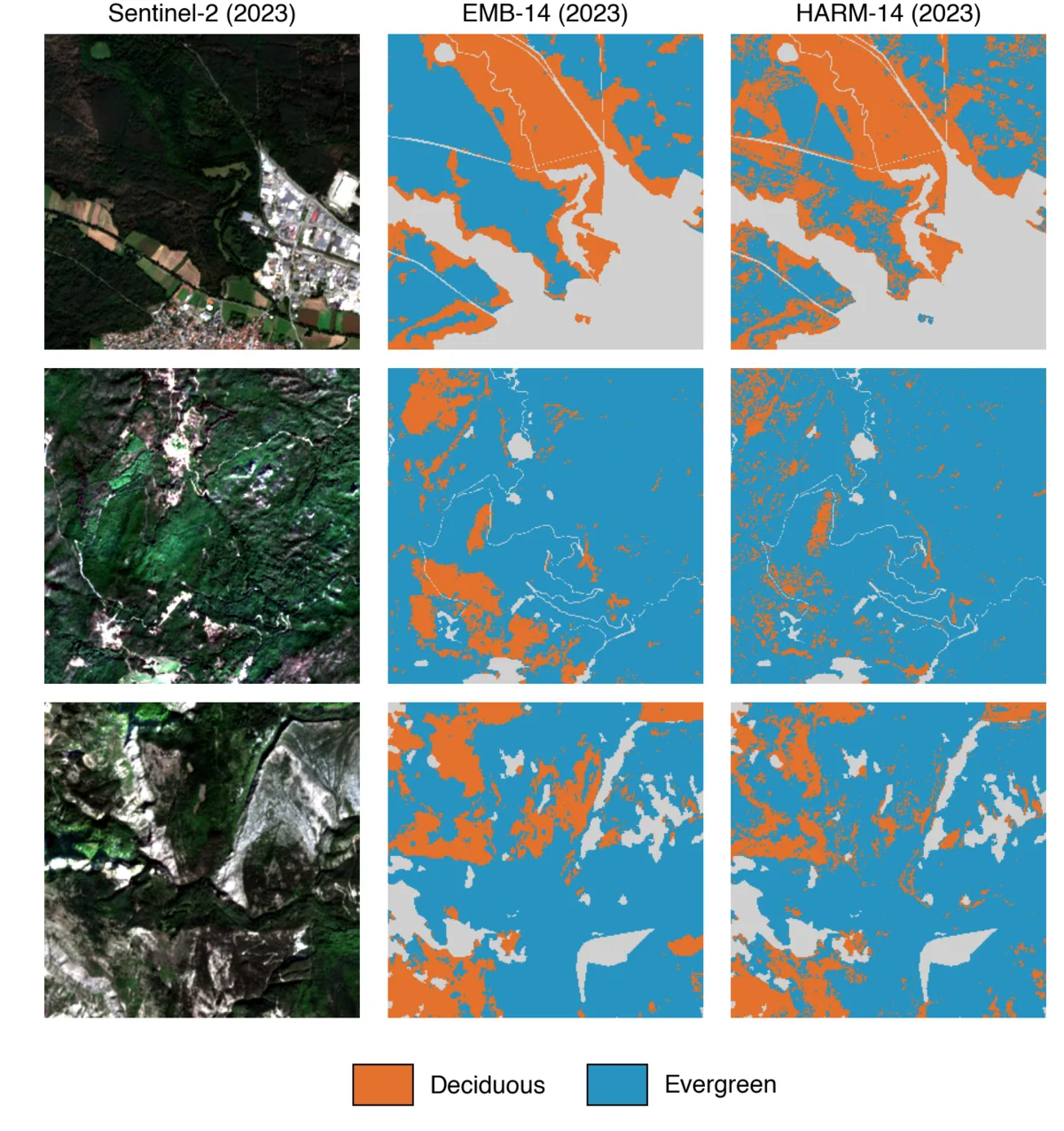
The largest improvements appeared in heterogeneous western and mountain regions: the Pyrenees gained 10.8 macro-F1 points and Corsica 8.8. Mediterranean France improved by only 0.7 points. Mediterranean conditions complicate the binary label: evergreen broadleaves break the broadleaf-conifer shortcut, while dry summers and autumn understory green-up can blur canopy seasonality at 10 m.
The harder problem was the reference data
The embeddings reduced the need to design seasonal features by hand, but they did not remove uncertainty from the labels. Models trained only on the geographically sparse field and expert labels transferred less well to BD Forêt than the reverse. Pooling both label families was the most robust strategy nationally.
A comparison with BD Forêt and Copernicus Dominant Leaf Type maps gave agreement around 0.63 for both embedding and harmonic predictions. This was a consistency check, not independent validation: BD Forêt contributed to training, the products were made in different years, and Copernicus maps broadleaf versus conifer rather than deciduous versus evergreen.
The manuscript also contains a temporal portability check. A random forest trained on 2023 embeddings was applied to 2018, 2020, and 2022 embeddings. Overall accuracy was 2.9 to 3.4 points lower than the 2023 training-set baseline, while the maps remained broadly stable. Because that baseline was not cross-validated, I treat this as a practical diagnostic rather than a performance claim.
The practical conclusion is modest. For this task, precomputed embeddings replaced much of the manual feature engineering and worked with ordinary classifiers on standard CPU infrastructure. That shifts more of the work toward sampling, label curation, regional validation, and uncertainty. This remains one foundation model, one binary task, and one country; it should not be generalized beyond that setting without further validation.