A land-cover map can look correct on one date and still be useless for measuring change. If a field moves from crops to grass because the next image was taken after harvest, or under a different haze, a downstream system may record an event that never happened.
During my 2022 internship at Kayrros, I revisited the nine-class problem used by Dynamic World, the 10 m near-real-time land-cover product developed by Google and WRI. Its Earth Engine collection provides probabilities for nine land-cover classes for individual Sentinel-2 observations. My narrower question was: which training and architecture choices make a sequence of these maps stable enough to support change analysis? This was an internal research and production project, not a claim to outperform Dynamic World as a global product.
Internship at Kayrros, supervised by Aurélien De Truchis.
Teach the model what should remain stable
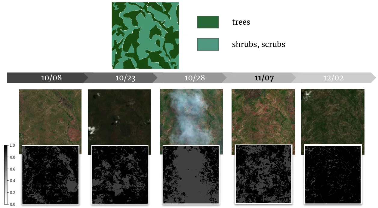
The Dynamic World paper tied each dense annotation to a Sentinel-2 image from one date. I turned each of those static examples into a small time series by retrieving other Sentinel-2 images from the 90 days before and after the annotation date.
The label stayed the same, but its confidence did not. For each date, I built a soft confidence map from Sentinel-2’s scene classification layer and four spectral indices: NDVI, NDMI, NDWI, and NDBI. Cloudy pixels and class-index combinations that looked implausible received less weight. Dates closer to the original annotation were sampled more often.
This did not tell the model that every nearby image was equally true. It asked the model to retain the land-cover signal while becoming less sensitive to clouds, colour, moisture, and seasonal vegetation changes.
The model used six optical bands shared by Sentinel-2 and Landsat: red, green, blue, near-infrared, and two short-wave infrared bands. It also used spectral indices and terrain derived from SRTM30. The reported experiments used Sentinel-2; adaptation to Landsat remained unfinished.
Change one part at a time
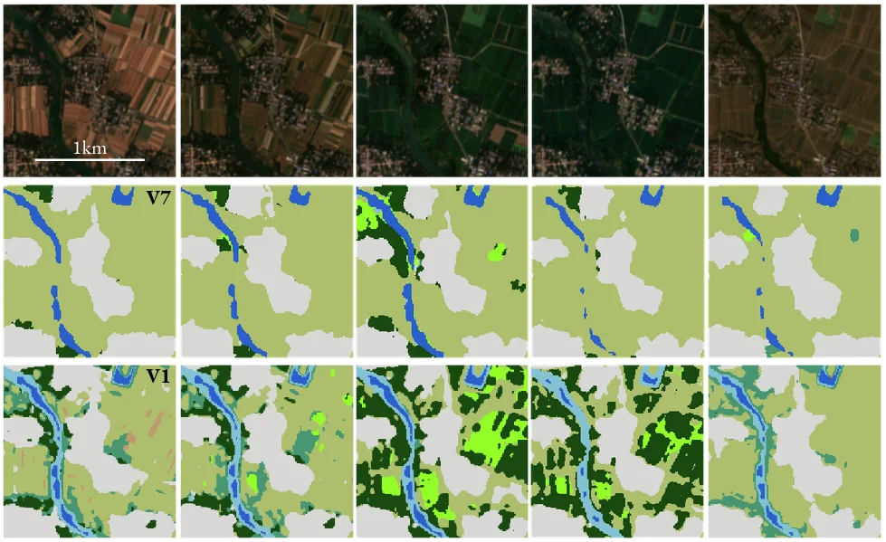
I tested nine versions under the same training setup. Some replaced the usual skip connections with dedicated paths for RGB texture, spectral indices, and elevation. Others added attention, MultiRes blocks, or Atrous Spatial Pyramid Pooling (ASPP) to give the model more spatial context.
V1, V7, and V8 are internal labels for this ablation study. They are not releases of the public GOOGLE/DYNAMICWORLD/V1 dataset.
- V1 was a three-level U-Net with classical skip connections filtered by attention gates. It recovered detailed edges, but reacted strongly to changes in colour, atmosphere, and season.
- V7 kept the attention gates and separated RGB texture, spectral indices, and terrain into dedicated paths. MultiRes blocks added multi-scale context in those paths and the decoder, with dropout at 0.2. It produced coarser maps, but the best temporal stability and balance across classes and biomes.
- V8 kept the attention gates and the three feature paths, but used ASPP instead of MultiRes blocks and removed dropout. It led on aggregate accuracy, intersection over union, and Matthews correlation, but was less balanced and sometimes produced checkerboard artefacts.
The compact U-Net I trained had about 1.6 million parameters. The larger alternatives we were comparing it with were around 20 million. That difference mattered because the model had to run repeatedly over large areas and many dates. Efficiency was part of the system design, not just a smaller number on a model summary.
The maps also had to remain readable at pixel level. The aligned view below shows one area near Mount Kenya: the satellite composite and the V7 prediction occupy exactly the same frame, so field boundaries and errors can be inspected directly.
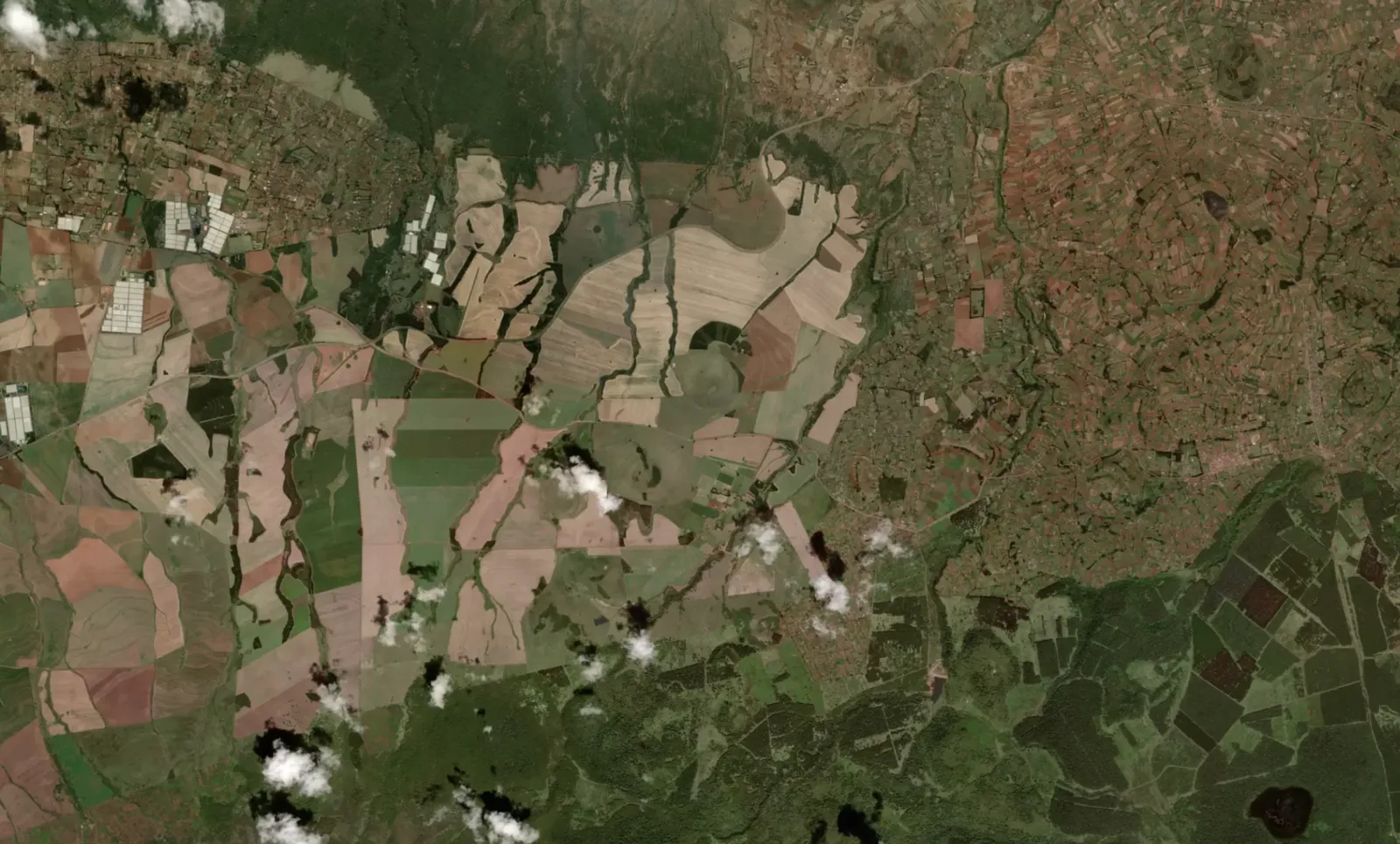
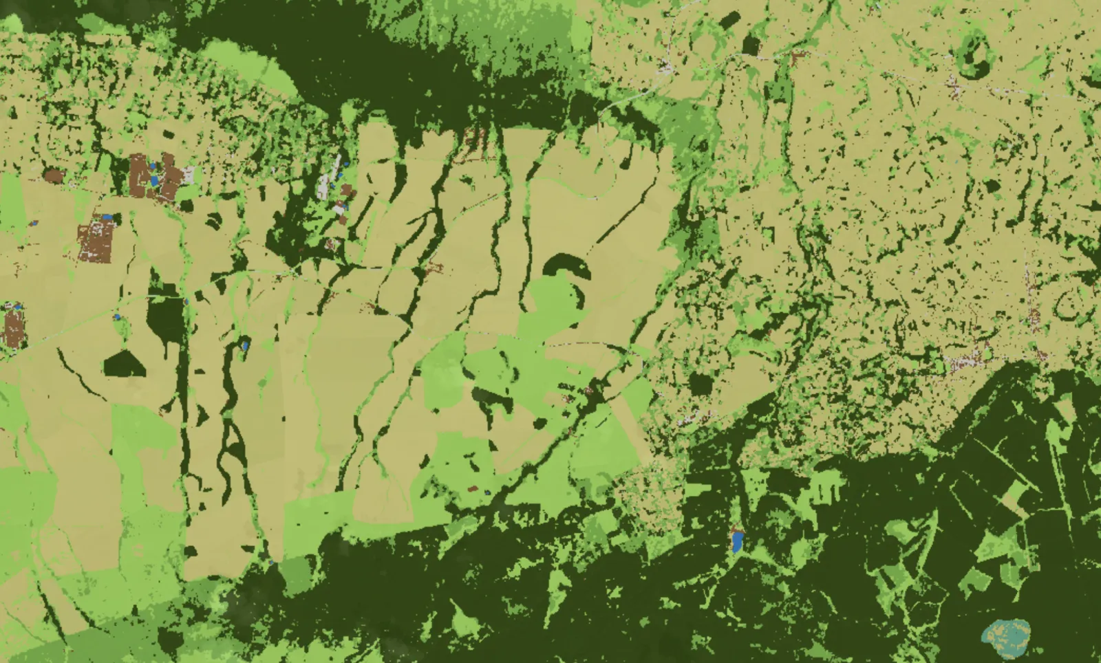

Evaluation used 1,300 areas of 5 by 5 km, labelled by consensus between three experts and spread across 14 biomes. I looked at overall accuracy, mean intersection over union, Matthews correlation, class and biome balance, and a separate stability test across dates.
The versions did not improve along one clean axis. V8 won on the aggregate metrics, while V7 was the more stable and balanced model. The right choice depended on what happened after classification.
That trade-off was the main result for me. If the output feeds a time series, the sharpest single-date map is not necessarily the most useful one. Detail, aggregate accuracy, balance, and temporal stability need to be measured separately.
From classifications to change signals
For the operational experiments, I filtered poor observations, aggregated class probabilities across dates, and compared the resulting maps through time. A qualitative test in Amazonia converted repeated land-cover predictions into a map of the first observed change date.
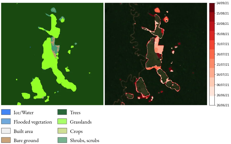
Some observed patches covered only three or four Sentinel-2 pixels, roughly 300–400 m². I would not present that as a validated detection limit. The result remained sensitive to weather, and I had not yet compared it properly with a purpose-built forest-loss alert system such as the University of Maryland’s GLAD forest alerts.
The project did reach production use in two biomass-related studies, but several research questions remained open: Landsat transfer, weak labels around small objects and borders, and independent validation of the change detector.
The lasting lesson was simpler. When a model sits inside a monitoring system, evaluation must follow the system’s purpose. For change detection, consistency across time is part of accuracy, not an optional extra.